Random Intercept Model in R: Interpretation and Visualization

A random intercept model in R is a useful tool for analyzing data from experiments that involve repeated measurements of the same participants or items. It allows you to control for the variability in the outcome variable due to random effects, such as individual differences or item difficulty, while estimating the fixed effects of your predictors of interest. In this blog post, will learn how to perform and visualize a random intercept model in R using a working memory example.

Outline

In this tutorial, we will learn:

The prerequisites for running a random intercept model in R include installing and loading the necessary packages and preparing your data.
How to carry out a random intercept model in R using the lmer() function from the lme4 package and interpret the output from the lmerTest package.
How to visualize a random intercept model in R using the plot_model() function from the sjPlot package, and how to customize the plots to suit your needs.

Prerequisites

You will need to install and load some packages to run a random intercept model in R. The most popular package for mixed effects models is lme4, which provides the function lmer() to fit the models. You will also need the lmerTest package, which adds p-values and degrees of freedom to the output of lmer(). To visualize the model, you will need the sjPlot package, which provides the function plot_model() to create various types of plots. You can install and load these R packages with the following code:

# Install the packages
install.packages(c("lme4", "lmerTest", "sjPlot"))
# Load the packages
library(lme4)
library(lmerTest)
library(sjPlot)Code language: R (r)

You will also need some data to work with. For this tutorial, I will use a simulated dataset that contains the results of a working memory experiment. Note you will also need to install dplyr, tibble, and tidyr to use the code to simulate data.

Simulated data

The dataset has four variables:

subject: the identifier of the participant (1 to 100)
item: the identifier of the memory item (1 to 20)
load: the memory load condition (low or high)

recall: the number of items correctly recalled (0 to 10)

We can create the dataset with the following code:

library(dplyr)
library(tidyr)
library(tibble)

# Seed for reproducibility
set.seed(20240711)

# Sample and Item size
n_subjects <- 125
n_items <- 20

# Tible ibble for subjects and items (can use data.frame as well)
subjects <- tibble(subject = 1:n_subjects)
items <- tibble(item = 1:n_items)

# Load conditions
load_conditions <- c("low", "high")


# Function to simulate working memory recall scores
simulate_recall <- function(load, subject_effect, item_effect) {
  if (load == "low") {
    rpois(1, lambda = 7 + subject_effect + item_effect) 
  } else {
    rpois(1, lambda = 4 + subject_effect + item_effect) 
  }
}

# Random effects for subjects and items
subject_effects <- rnorm(n_subjects, mean = 0, sd = 1)
item_effects <- rnorm(n_items, mean = 0, sd = 0.5)

# Create the dataset by combining subjects, items, and load conditions
data <- subjects %>%
  crossing(items) %>%
  mutate(load = sample(load_conditions, n(), replace = TRUE)) %>%
  rowwise() %>%
  mutate(
    subject_effect = subject_effects[subject],
    item_effect = item_effects[item],
    recall = min(max(simulate_recall(load, subject_effect, 
                                     item_effect), 0), 10)
  ) %>%
  ungroup() %>%
  select(subject, item, load, recall)Code language: R (r)

In the code chunk above, we used tibble to create a dataframe. Moreover, we used select() to select columns by their name (i.e., the ones we need in our dataframe). The tibble, dplyr, and tidyr packages are useful for data manipulation tools such as adding columns to dataframes, removing columns, and convert data from wide to long. Note that when working with your own data you need to have it in long format.

How to carry out a random intercept model in R

To fit a random intercept model in R, we can use the lmer() function from the lme4 package. The syntax of the function is:

lmer(formula, data)Code language: R (r)

where formula is a formula object that specifies the fixed and random effects of the model. Moreover,data is the dataframe that contains our variables in the formula.

The formula object has the following general form:

outcome ~ fixed + (random | grouping)Code language: R (r)

where outcome is the name of our outcome/dependent variable. Moreover, fixed is a list of our fixed effects separated by + signs, and random is a list of our random effects separated by + signs. Finally, grouping is the name of the variable that defines the levels of the random effect.

For example, to fit a random intercept model for the simulated working memory data, where the outcome variable is recall, the fixed effect is load, and the random effects are subject and item, we would use to following formula:

recall ~ load + (1 | subject) + (1 | item)Code language: R (r)

We can pass this formula to the lmer() function along with the dataframe to fit the model:

library(lmerTest)
model <- lmer(recall ~ load + (1 | subject) + (1 | item), data)Code language: R (r)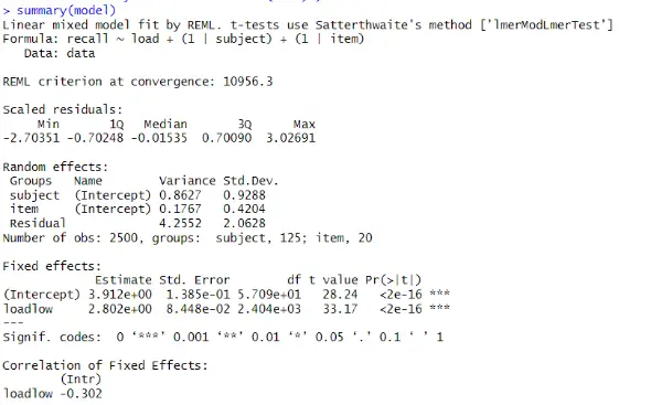

getting the results from a random intercept model in R

Interpretation

We can see the estimated fixed and random effects, as well as their standard errors and significance tests, in the output. We interpret them as follows:
The fixed effects show the main effects of the predictor variable load on the outcome variable recall. The intercept is the estimated mean recall score when load is high, which is 3.912. The coefficient of loadlow is the estimated difference in recall score between low and high load, which is 2.802. This means that we recalled more words when the load was low than when it was high. Both the intercept and the coefficient of loadlow are significant, as the p-value is less than 0.05, indicating a load effect on recall.
Furthermore, the subject variance is the estimated variability in the intercepts across the subjects after accounting for the fixed effect of load. It is 0.98, meaning variation in the participants’ baseline memory capacity exists. Next, we can se the item variance which is the estimated variability in the intercepts across the items after accounting for the fixed effect of load. It is 0.24, which means there is some variation in the items’ difficulty.
The residual variance is the estimated variability in the recall scores not explained by the fixed or random effects. It is 3.79, meaning there is still a lot of noise in the data.

How to visualize a random intercept model in R

We can use the plot_model() function from the sjPlot package to visualize a random intercept model in R. This function can create various plots, such as forest plots, marginal effects plots, or slope plots, depending on the type argument. For example, to create a forest plot that shows the confidence intervals of the fixed and random effects, we can use the following code:

plot_model(model, type = "re")Code language: R (r)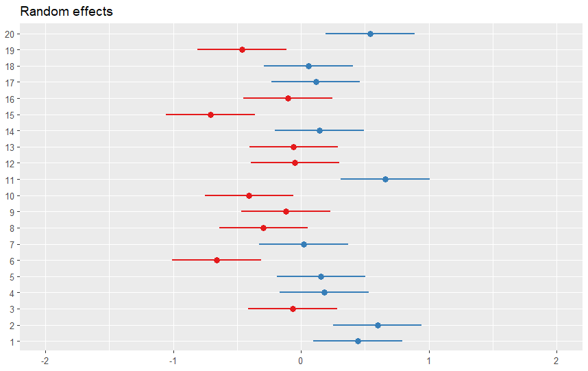

random intercept model in R with the random effects (item) plotted

Customizing the Plot

One neat thing is that the output of the plot_model() function is a ggplot object, which means that you can customize the plot using the functions and arguments from the ggplot2 package. For example, to change the title, labels, and colors of the plot, we can use the following code:

library(ggplot2)
pm <- plot_model(model, type = "re") 

pm[[2]] + 
  labs(title = "Random intercept model for working memory data",
               x = "Effect size",
               y = "Random effects (item)") Code language: R (r)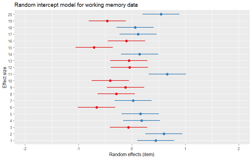

Customizing APA 7 and Saving the Plot in High Resolution

To customize the plot (i.e., the pm object) to follow APA 7 we can use the following code:

# Customize the plot to follow APA 7th edition guidelines
custom_plot <- pm[[2]] + 
  labs(
    title = "Random Intercept Model for Working Memory Data",
    x = "Item Number",
    y = "Random Effects (Item)"
  ) + 
  theme_minimal(base_size = 12, base_family = "sans") + 
  theme(
    plot.title = element_text(face = "bold", size = 14, hjust = 0.5), 
    axis.title.x = element_text(face = "bold", size = 12),
    axis.title.y = element_text(face = "bold", size = 12), 
    axis.text = element_text(size = 10), # Axis text size
    panel.grid.major = element_blank(), 
    panel.grid.minor = element_blank(), 
    panel.border = element_blank(), 
    axis.line = element_line(linewidth = 0.5, colour = "black"), 
    legend.position = "none" 
  )Code language: R (r)

In the code chunk above, we used theme_minimal() and theme() to create an APA 7 style plot of the random intercept model, showcasing the random effects. We started with theme_minimal(base_size = 12, base_family = "sans") to provide a clean base theme, setting the base font size to 12 and using a sans-serif font for compatibility. We customized the plot title using plot.title = element_text(face = "bold", size = 14, hjust = 0.5), making it bold, setting the font size to 14, and centering it. For the x and y axis titles, axis.title.x and axis.title.y were set to bold with a font size of 12 using element_text(face = "bold", size = 12). We ensured readability of axis text with axis.text = element_text(size = 10).
To remove grid lines, we used panel.grid.major = element_blank() and panel.grid.minor = element_blank(). We eliminated the panel border with panel.border = element_blank(). To add axis lines, we applied axis.line = element_line(linewidth = 0.5, colour = "black"), setting the line width and color. Lastly, we removed the legend by setting legend.position = "none".

To save the plot as a high -resolution TIFF we can use this code:

# Save the plot as a high-resolution TIFF file with 300 DPI
ggsave("custom_plot.tiff", plot = custom_plot, dpi = 300,
       width = 8, height = 6, units = "in")Code language: R (r)

Report Correlation in APA Style using R: Text & Tables

Note that we can also plot the fixed effects including interactions using plot_model.

Summary: Random Effects Model in R

In this blog post, you learned how to run and visualize a random intercept model in R. A random intercept model is a mixed effects model that allows you to account for the variability in the outcome variable due to random effects, such as participants or items. We learned how to use the `lmer()` function from the lmerTest (lme4( package to fit the model, how to interpret the output from the lmerTest package, and how to use the `plot_model()` function from the sjPlot package to create different types of plots. Finally, we also learned how to customize the plots using the ggplot2 package.

I hope you found this tutorial helpful and informative. If you did, please share it with your friends and colleagues who might be interested in learning more about mixed-effects models. If you have any questions or comments, feel free to leave them below.

R Tutorials

Here are some more analysis-related tutorials on this blog:

Correlation Matrix in R: A Hands-On Guide for Practical Analysis

Master MANOVA in R: One-Way, Two-Way, & Interpretation