In a previous post, we learned how to use Binder and Python for reproducible research. Now, we are going to learn how to create a Binder for our data analysis in R, so it can be fully reproduced by other researchers. More specifically, in this post, we will learn how to use Binder for reproducible research.
Many researchers upload their code for data analysis and visualization using git (e.g., GitHub, Gitlab).
No doubt, uploading your R scripts is great. However, we also need to make sure that we share the complete computational environment so that our code can be re-run and so that others can reproduce the results. That is, to make sure that other researchers really can reproduce our code, we need a way to capture the versions of the R packages we used when publishing our research.
As previously, mentioned, uploading the R scripts, the data, and sharing the links to the online repositories (e.g., GitHub or the Open Science Framework) is a good start. Recreating, however, the exact environment, including the versions used when analyzing data, required to run another researcher’s analysis may involve a lot of time. That is, if another researcher wants to conduct the exact same analysis, using the same versions, that researcher needs to install the R version, the versions of the packages, and so on, before conducting the reproducibility analysis.
Luckily, there are some alternatives to help us with creating reproducible environments. For example, Binder and Code Ocean can make a difference; these tools enable us to reproduce our exact R statistical programming environment, with an online RStudio. This, in turn, will enable other researchers to reproduce our exact workflow, as well as change it. The end product, sort of speak, is an online repository with the R environment we used. In this online environment, data analysis can be re-run by other researchers. It is, also, possible for them to change things around in the scripts. Note, however, any changes are not saved to the scripts.
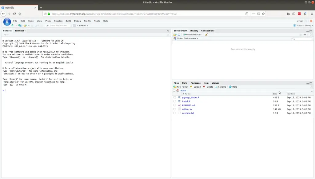
Table of Contents
- What is Binder
- How to Use Binder for Reproducible Code
- How to Use Git
- How to Create a Reproducible R Environment
- Connecting Everything to Binder
- Summary
- More Resources
What is Binder
In this post, the focus is on Binder and how to use Binder for reproducible research. That is, the post will not cover any technical details about Binder.
However, this section will shortly cover what Binder is. Binder makes it possible for us to create custom computing environments. Furthermore, these computing environments can be shared and used by many other researchers. For example, the exact data analysis can be run, by another scientist, by following a link to RStudio that can be run in a web browser. Finally, Binder is powered by BinderHub, an open-source tool that deploys the Binder service to the cloud.

In this R and Binder tutorial, we will use mybinder.org. You may now ask yourself: how does Binder work? Binder is pulling a repository, that we set up on GitHub into a Docker container. After this, Docker packages our data, code, and all the dependencies, specified in a file, into a docker container. Finally, this ensures that our scripts work seamlessly in any environment.
How to Use Binder for Reproducible Code
In this Binder tutorial, we will create a scatter plot on a map and use it when we create our Binder repository. Here, we use the following tools and r-packages:
All packages above can be installed on our computers using the following r code:
list.of.packages <- c("ggplot2", "ggmap", "osmdata")
new.packages <- list.of.packages[!(list.of.packages %in%
                                     installed.packages()[,"Package"])]
if(length(new.packages)) install.packages(new.packages)Code language: R (r)
Note, the above r packages will be installed when we create the Binder but, typically, we also want to use them locally, on our computers. Notice how we created a character vector with the packages and then used R’s %in% operator to match values between this vector and the installed packages. A quick note, before moving on, ggplot2 is part of the Tidyverse package. This means that you can install this package and get ggplot2 among other useful packages. For example, you can use dplyr to rename a column in R, add a column to a dataframe based on other columns, and rename factor levels, among other things.
How to Use Git
In this post, on how to use Binder for reproducible code, we are going to use the command line application called git. Thus, we need to create a GitHub account and install Git. If you already know how to use Git, click here to skip this part.
In the git example below, we are using Ubuntu 18.04, and a terminal prompt. If you are a Windows user you can see how to use git and git bash in the Binder and Python tutorial.
Step 1: Install Git and Set it Up

Open up a terminal window and type code apt install git
When git is installed, we need to configure git.
In the terminal window, we type:
git config --global user.name "Your name here"
git config --global user.email "your_email@example.com"Code language: Bash (bash)
Step 2: Create a GitHub Repository
Now that we have git installed, we are going to create a directory for our repository. Let’s open up the terminal window, again. In the terminal window, we type the following commands:
cd Documents
mkdir Binder
cd Binder
mkdir bindRtut
cd bindRtutCode language: Bash (bash)
The next thing to do is to initialize the git. This is easy, and we type one command in the terminal window:
git initCode language: R (r)Step 3: Create the environment and a README files
In the next step, we are going to create our runtime.txt and README.md files. The file runtime.txt is where we tell which R environment we will use (the date we ran the script). This way, when we later create the Binder, we are going to create a “time machine” with the R version from this date.
Creating the runtime.txt file:
First, we open up a text editor, in this case, we’ll use RStudio to create a new file (New File > Text File):
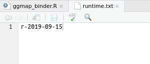
Of course, you can use any other text editor to create a text file (e.g., Notepad).
When this is done, we are going to save this file as “runtime.txt” in the directory we already have created.
Creating the install.R File
We also need to create the install.r file to tell Binder to install the r-packages we use in our script. Again, File New > New Rscript and save this file as “install.r”, in the folder we previously created. Note, here, it’s very important that we add all the packages we used, or else the scripts will not run in our Binder. Add the command below to that file.
install.packages(c("ggplot2", "ggmap", "osmdata"))Code language: R (r)Creating the README.md file:
In RStudio, we will now create another file: File New > New R Markdown and select From Template and GitHub Document (Markdown). Finally, save this file in the same directory as the runtime.txt, README.md, and add the following text:
## How to Use Binder for Reproducible Research
Example README.md file for the tutorial on how to use Binder for reproducible research in R statistical environment.
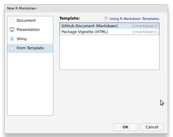
Note, the above is an example README.md file created for the tutorial on how to use Binder for reproducible research in R. Naturally, for a real science project, we would have a more detailed description of the study, methods, and statistical analysis in the README.md.
- How to Transpose in R with the t() Function – matrix and dataframe
- How to Get Absolute Value in R – vector, matrix, & data frame
Step 4: Add the Files and Create a Commit
Finally, we are ready to commit our files to GitHub. Let’s open up a terminal window. Remember to change the directory to the right one and type:
git add .
git commit -m "Created the binder r environment, install.r, and README files"Code language: Bash (bash)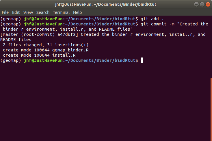
Step 5: Create a new repository on GitHub
In the fifth step, we are going to create a new repository on GitHub.
First, we go to the GitHub home page and press the green ‘+ New repository button:

After we have clicked the button, GitHub will ask us to name the repository. In this Binder example we leave out the description and give the repository the name “bindertut”:
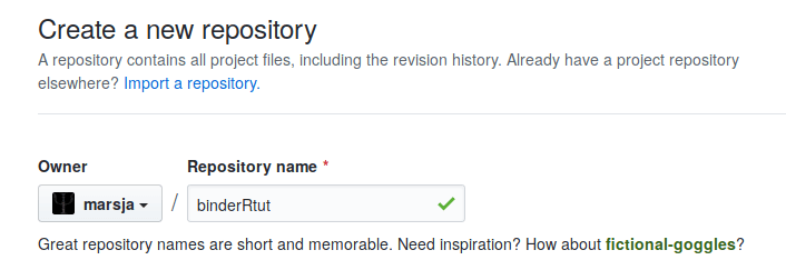
In this Binder tutorial, we only fill in the repository name and we can now press the green ‘Create repository’ button to make our new repository.
Note, we have already created a new repository locally and, thus, we want to push that onto GitHub. First, we open up the terminal window again and type the git commands below.
git remote add origin git@github.com:marsja/binderRtut.git
git push -u origin masterCode language: Bash (bash)
Remember, we need to be in the same directory where we have initialized Git and store all the files (e.g., README.md, R-scripts).
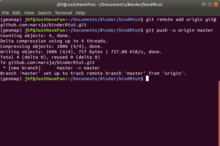
Note, remember to change the username (i.e., marsja to yours). For more guides on how to use Github see here.
How to Create a Reproducible R Environment
In the next code example, we are going to create a scatterplot of Google location history data (your data can be downloaded from your Google account, but the data need to be pre-processed before using the R script below).
R Code Example:
In the R code example below, we start by loading the ggmap and osmdata libraries. In the next step, we get the map data for Rotterdam. Finally, we read the pre-processed data of GPS coordinates from a visit to Rotterdam and print the first 5 rows using head().
library(ggplot2)
library(ggmap)
library(osmdata)

# Getting data for Rotterdam
rotterdam <- getbb('Rotterdam')

df <- read.csv('rotter.csv')

head(df)Code language: R (r)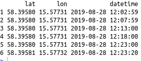
In R, data can be imported from many formats. If the data is stored in Excel files, it is possible to use the readxl and xlsx packages to load the data into R dataframes. Learn more about working with Excel files in the recent R Excel tutorial. As you can see, in the image above, there are dates down to the seconds in one of the columns above. If you want to visualize the data in hour, days, or year check the following tutorials:
- How to Extract Time from Datetime in R – with Examples
- How to Extract Day from Datetime in R with Examples
- How to Extract Year from Date in R with Examples
Additionally, sometimes when we import data in R we don’t want all the columns in the dataset. Now, that leads to that we may want to use dplyr to remove a column in R (or many columns, of course). Furthermore, we may need to clean the data frame from duplicate rows, in some cases.
Learn more about different operators in R:
- How to use $ in R: 6 Examples – list & dataframe (dollar sign operator)
- How to use %in% in R: 7 Example Uses of the Operator
Scatter Plot on a Map
In the next code example, we create a scatterplot using ggplot2 and ggmap. First, we start by using the get_map function to get the coordinates of Rotterdam. Here, we zoom in at 13 and use the source “osm”. Next, we create the map using ggmap and the coordinates (i.e. rott). Finally, we create the scatter plot in R using the function geom_point. In this function, we use the lon and lat columns from the dataframe, df.
rott <- get_map(rotterdam, zoom = 13, source = "osm")

ggm <- ggmap(rott, extent="device", legend = "none")

ggm <- ggm + geom_point(aes(x = lon,  y = lat),  data = df)

print(ggm)Code language: R (r)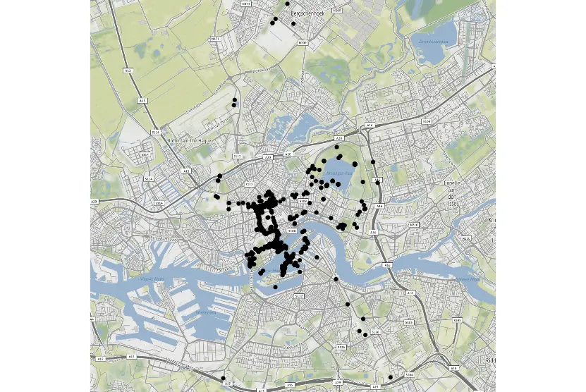
Scatter plots in R is easy to create. In another blog post, we learn how to use ggplot2 to make beautiful scatter plots. This tutorial is very extensive, and we will learn how to change the axis ticks, and save the plots in high-resolution files, among many other things:
Finally, it’s time to upload our code to Binder. First, we need to push this to git. As in the previous steps we open up the terminal window (make sure to be in the correct directory), and we use the following commands:
git add .
git commit -m 'Added data vis'
git push -u origin masterCode language: Bash (bash)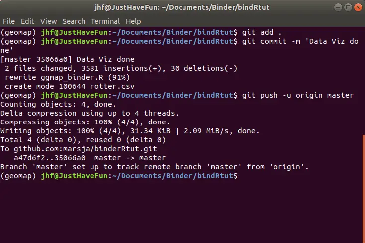
Here are some more R tutorials that you may find useful:
- How to Create Dummy Variables in R (with Examples)
- How to use the Repeat and Replicate functions in R
Connecting Everything to Binder
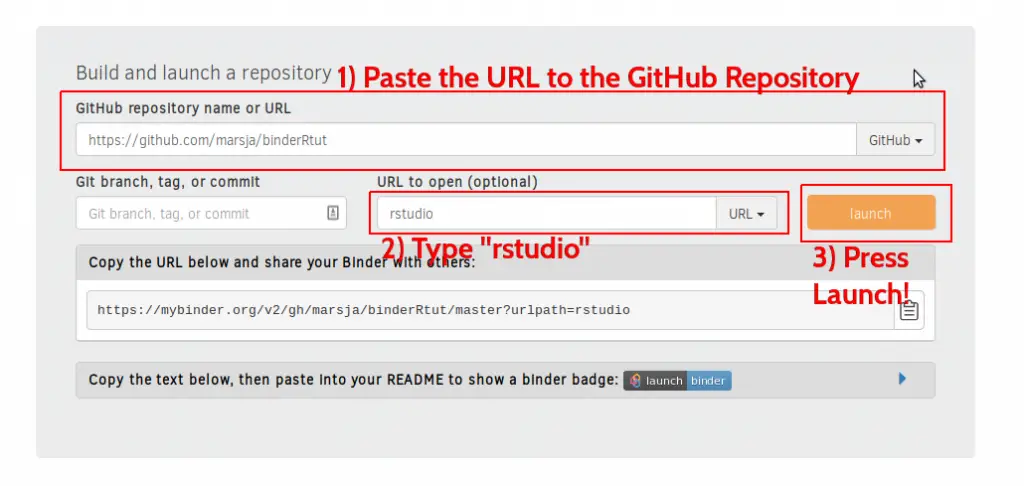
Finally, we are ready to create our Binder. This is quite easy, we open up a new tab in our browser, type “https://gke.mybinder.org/” and hit enter.
How to Create a mybinder in 3 Simple Steps
Time needed: 1 minute
How do you create a Binder using mybinder? Here are three simple steps:
- Paste URL to GitHub Repository
First, we paste the URL to the GitHub Repository we created
- Type “rstudio”
In the form, where it says “Path to a notebook file (optional”) type Rstudio
- Press “Launch”
Now we are ready to launch the Binder
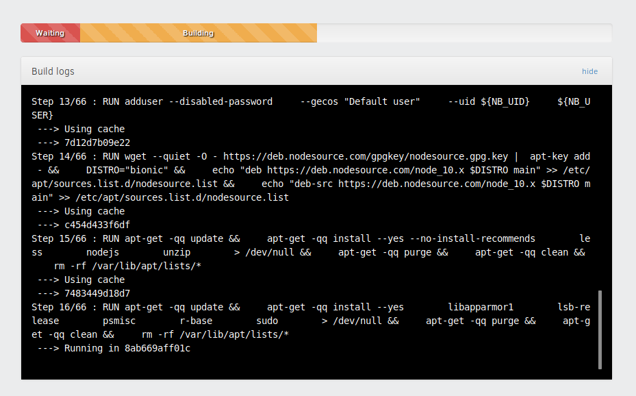
Now we can sit back, have a beer, and wait for it to be done. The process of building everything may take a long time. After everything is done we’ll get a link to share with other researchers.
Finally, it’s important to remember that any changes in the RStudio online, on mybinder.org, will not be saved. In fact, the RStudio will automatically shut down after 10 minutes of inactivity. Of course, the Binder can be updated. In fact, all we need to do is go back to our repository, make changes, commit, and push back to GitHub.
Note, for Windows users please have a look at the how-to-use Git section in the tutorial on how to use Python and Binder. In Windows, we can use Git Bash instead of a Linux terminal window.
Summary
In this tutorial, we have learned how to set up git, use GitHub together with Binder for Reproducible data visualization. Furthermore, we used ggplot2, ggmap, and osmdata for visualizing Google location data in RStudio. This RStudio online, along with the GitHub repository we created, can be found online here.
More Resources
Here are some more resources that you may need:
- Correlation in R: Coefficients, Visualizations, & Matrix Analysis
- How to Create a Sankey Plot in R: 4 Methods
- Report Correlation in APA Style using R: Text & Tables
- Binning in R: Create Bins of Continuous Variables


